By the end of this lecture, you should be able to formally define what a limit is, using precise mathematical language, and to use this language to explain limit calculations and graphs which we completed in previous sections.
So far we have worked with an informal definition of the limit:
Limit (informal definition)
If f(x) eventually gets closer and closer to a specific value L as x approaches a chosen value c from the right, then we say that the limit of f(x) as x approaches c from the right is L.
If f(x) eventually gets closer and closer to a specific value L as x approaches a chosen value c from the left, then we say that the limit of f(x) as x approaches c from the left is L.
If the limit of f(x) as x approaches c is the same from both the right and the left, then we say that the limit of f(x) as x approaches c is L.
If f(x) never approaches a specific finite value as x approaches c, then we say that the limit does not exist. If f(x) has different right and left limits, then the two-sided limit (limx→cf(x)) does not exist.
Notation:
Specifically, we write:
limx→c-f(x) = L to denote "the limit of f(x) as x approaches c from the left is L"
limx→c+f(x) = L to denote "the limit of f(x) as x approaches c from the left is L"
limx→cf(x) = L to denote "the limit of f(x) as x approaches c is L"
However, this definition is informal because we haven't formally defined what we mean by "approaches" or "eventually gets closer and closer to". In order to come up with a formal definition, we will need to clarify exactly when we can say that x or f(x) approach a specific value. We do this now by providing a formal mathematical definition:
Limit (formal definition)
Finite Limits:
If f(x) is a function that is defined on an open interval around x=c, and L is a real number, then
limx→cf(x) = L
means that:
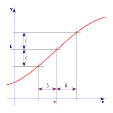
For any number ε>0 that we choose, it is possible to find another number δ>0 so that:
for all x's between c-δ and c+δ (except possibly at c exactly), f(x) will fall between L-ε and L+ε.
In other words, if we pick an interval on the y-axis around L, we can always find an interval on the x-axis around c that will force f(x) to stay with the chosen range of y-values (except for perhaps at f(c)). This is probably best understood by looking at a graph:
If we want a formal defintion of what it means for a limit to increase or decrease without bound, we can also adapt this approach to this case:
Infinite Limits:
If f(x) is a function that is defined on an open interval around x=c, then
limx→cf(x) = +∞
means that:
For any number M>0 that we choose, it is possible to find another number δ>0 so that:
for all x's between c-δ and c+δ (except possibly at c exactly), f(x) will be greater than M.
In other words, if we pick a value on the y-axis around, we can always find an interval on the x-axis around c that will force f(x) to stay above this value (except for perhaps at f(c)). This is probably best understood by looking at a graph:
We can also use this same idea to create a definition for limits at infinity:
Limits at Infinity:
If f(x) is a function and L is a real number, then
limx→∞f(x) = L
means that:
For any number ε>0 that we choose, it is possible to find another number M>0 so that:
for all x's greater than M, f(x) will fall between L-ε and L+ε.
In other words, if we pick an interval on the y-axis around L, we can always find a cutoff value on the x-axis that will force f(x) to stay with the chosen range of y-values once it is past this cutoff location. This is also probably best understood by looking at a graph:
So, if a limit exists, it should be possible to bound an area around c that will force f(x) to stay within any chosen specific distance of L. Let's see how this definition can be applied to the example limit calculations that we've done in previous lectures. In cases where the limit does not exist, we should be able to see why a δ won't exist for every possible ε: in other words, we should be able to find an ε in these cases for which no possible δ can be found which will force f(x) to remain within a distance ε of L.
Limits of Specific Functions
For each of the following examples, we look at how the formal definition of the limit allows us to prove that the limit exists or that it does not exist. We do this both by using graphs to see if we can approximate the appropriate values for δ or M, and by seeing if we can calculate these values exactly by approaching the equation algebraically.
A simple example, where limx→cf(x) = f(c):
For this function, we are interested in the limit as x approaches 1:
We have already calculated this limit both graphically and algebraically and determined that it is 2. But now we'd like to use the formal definition of the limit to better understand why the limit exists. To do this, we are going to find the δ value(s) that will fulfil the requirements of the limit defintion for ε=0.05.
To do this graphically, we can move the ε slider on the interactive animation below until it reachers 0.05. Then we can move the δ slider until the dotted green lines that represent the part of the graph where all points are within a δ-distance or less from x=1. Once these green dotted vertical lines are close enough together to ensure that all of f(x) in between stays inside the red shaded portion of the graph, we have found a δ that will keep f(x) within a distance of ε of the limit 2. At approximately which value of δ do the vertical green dotted lines keep the graph of f(x) within the red portion of the graph?
ε
δ
Interacting with the animation, you should have found that δ = 0.0248, or something close to this, seems to be sufficiently small to ensure that f(x) stays within a distance of 0.05 of the limit 2.
Now, to do this algebraically, we start by bounding f(x) by L-ε on the left and L+ε on the right, and then we solve this inequality for x. This allows us to determine which values of x will allow us to keep f(x) within a distance of ε from the limit 2:
So if x stays within 0.025 distance of c=1, f(x) will stay within 0.05 distance of L=2. (Of course, any δ smaller than 0.025 will also work!)
An example with a hole at x=c:
We are again interested in the limit as x approaches -2, and we recall from the last few lectures that the limit in this case is -4. In this problem, let's look for a δ that will work for ε=0.02.
To begin, we attempt to find the δ graphically by interacting with the animation below, which will give us an approximate value:
ε
δ
Interacting with the animation, I got a value of about 0.0206 for δ. What did you get?
Now, solving for δ algebraically to get an exact value:
An example with a function that has a jump discontinuity at x=c consisting of a single point:
We are again interested in the limit as x approaches -2, and we recall from the last few lectures that the limit in this case is -4. For this example, we again seek a δ which works for ε=0.02.
First we aim to estimate δ graphically, using the animation below:
ε
δ
We notice that this problem is really no different from the last one: the only difference here is that while the previous graph had a hole at x=2, whereas this graph, in addition to that hole, has an isolated point at (-2,1). But this has no effect on the limit because the limit is not concerned with what happens atx=c, but only what happens aroundx=c. So in this case, our previous δ=0.02 will still work, even though the point (-2,1) is not within 0.02 of -4. We should precisely exclude this point when looking at the limit, by definition.
In the next example, we will use the formal limit definition to evaluate one-sided limits, and before we do that, we want to briefly introduce a piece of notation that we will use:
Notation: LL and LR
We will use the notation LR to denote the limit calculated as x approaches c from the right, and we will use the notation LL to denote the limit calculated as x approaches c from the left.
An example with a function that has a jump discontinuity at x=c, and different limits from the right and from the left:
Here we are interested in the limit as x→1, and we will seek to find a δ that satisfies the formal limit defintion for ε=0.1. Since this is a piecewise function with a jump discontinuity at x=1, we will first look at the limit separately from the right and from the left:
First we consider the limit from the right, which we have already calculated in a previous lecture as 2. First we will estimate it graphically, using the interactive animation below, and then we will calculate it algebraically.
ε
δ
By using the sliders to set ε at 0.1, and then moving the slider for δ until the green dotted line on the right keeps the graph of f(x) to the left of x=1 within the red shaded area, I obtained an approximation of δ from the graph that was 0.0777. What did you get?
Now, calculating δ algebraically for the right-hand limit:
Now we consider the limit from the left, which we have already calculated in a previous lecture as -2. Again we will begin by estimating it graphically using the animation below, and then we will calculate it algebraically.
ε
δ
By using the sliders to set ε at 0.1, and then moving the slider for δ until the green dotted line on the left keeps the graph of f(x) to the left of x=1 within the red shaded area, I obtained an approximation of δ from the graph that was 0.037. What did you get?
Now we proceed to calculate the value of δ algebraically for the left-hand limit:
Now we consider the two-sided limit. If we try to use the formal defintion of the limit with a value of ε=0.1, we run into a problem: we cannot choose any δ that will always keep f(x) within an ε distance of the left-sided limit -2 on the left, because no matter how small we make our δ, there will always be a bit of the graph just to the right of x=1 where f(x) falls far outside of the area which is a distance of ε or less from the left-sided limit. Similarly, we cannot choose any δ that will always keep f(x) within an ε distance of the right-sided limit 2, because no matter how small we make our δ, there will always be a bit of the graph just to the left of x=1 where f(x) falls far outside of area which is a distance of ε or less from the right-sided limit.
In fact, we would need to have an ε of 4 or larger in order to force all of the f(x) values in the neighborhood of x=1 to be within an ε distance of both the left and the right limit values. But the formal defintion says that we must be able to find a δ for ALL possible non-zero choices for ε. So if we can find even one non-zero value for ε for which no δ is possible, we have shown that the limit does not exist.
An example with a function that has an infinite discontinuity (or vertical asymptote) at x=c:
For this function, we are interested in the limit as x approaches 0. We can see here that we will not be able to find a δ for any ε in this case which will work for a finite limit, because f(x) here is increasing without bound as x approaches 0 from either side. So in this case we will use the formal definition of infinite limits to find a value for δ when M=100.
We begin by approximating δ graphically: using the sliders on the interactive animation below.
M
δ
I obtained an approximate value of 0.095. What did you get?
Now, we solve for δ algebraically:
An example with a function that has an infinite discontinuity (or vertical asymptote) at x=c, with different limit behavior from the left and from the right:
For this function, we are interested in the limit as x approaches 1. Let's see now if we can find an appropriate δ for M=40 on the right side, and an appropriate δ for M=-40 on the left side, first by using the graph to approximate a value:
M
δ
M
δ
For both the left and the right, I obtained a value of δ=0.026, by using the sliders on the interactive animations above. What did you get?
Now let's calculate δ exactly algebraically. First we begin by finding which value of δ will keep f(x) above M (on the right-hand side).
Now we calculate which value of δ will keep f(x) below -40 (on the left-hand side).
We can see again why the two-sided limit does not exist in this case, because there is no possible δ that we could choose that would keep all the values of f(x) above 40 (because there would always be some values to the left of x=1 included, and they are all negative), no matter how small δ is. We would run into a similar problem with the positive values of f(x) to the right of 1 if we tried to find a δ which works for the two-sided limit when M=40 (because there would always be some values to the right of x=1 included, and they are all positive).
An example with a function that has a limit of zero at infinity:
For this function, we are interested in the limit as x approaches -∞ and the limit as x approaches +∞. We will look for values of M that will satisfy the formal limit definition when ε is equal to 0.45. Because of the relative complexity of this particular equation, we will only estimate the M values graphically, rather than verifying them algebraically in this case. Use the sliders in the interactive animation below to find an M for ε=0.45 for both limits:
ε
M
Looking at the limit as x approaches -∞, we obtain a value for M which is approximately 4.4, and looking at the limit as x approaches +∞ we obtain a value for M which is approximately 4.35.
An example with a function whose limit does not exist at infinity:
We consider the limit of this function as x approaches +∞, and we consider whether we can find an M for ε=0.5. Again, for this problem, because the equation is relatively complex, we use the animation to approximate values of M rather than trying to find M algebraically. Try experimenting with the sliders below to see if you can find a value for M which will keep the values of f(x) in the red shaded region for all x>M.
ε
M
We can see that in this example, it will never be possible to find such an M, because as x increases without bound, f(x) also increases without bound. No matter what value we choose for M, we will never be able to keep the graph of f(x) within the red shaded region.
An example with a function that has an oscillating discontinuity:
We consider the limit of this function as x approaches 1, and we aim to find a δ which will satisfy the formal limit definition for ε=0.5. This is another problem where will just look at the graph to try to find δ rather than also trying to find δ algebraically. Looking at the animations below, take some time to experiment with the sliders to see if you can find a δ for ε=0.5 for either a one-sided or two-sided limit at x=1.
ε
δ
ε
M
You have perhaps noticed that it is not possible to find such a δ, because no matter how small a δ you choose, there will always be some part of the graph inside the dotted green lines which oscillates up to 1 and down to -1. So there is no such value that will keep the graph of f(x) inside the red shaded area, and we can see how the formal definition of the limit shows us that this limit does not exist.