Estimating Instantaneous Rates of Change (Derivatives) Graphically
By the end of this lecture, you should be able to estimate instantaneous rates of change (or derivatives) graphically. If given a graph of a function, you should be able to draw a tangent line (i.e. the line whose slope is the instantaneous rate of change at that point) at a given point on the graph, and draw the graph of the derivative of the function. You should also be able to determine where the derivative of a graph might be zero, positive, negative, increasing, decreasing, or undefined. You should also begin to get a feeling for which types equations might represent the derivatives of different types of functions, based on the patterns you observe in the graphs.
In the introductory lecture for this course, we discussed a few of the questions that motivated the development of calculus. The first question, which motivated us to develop the theory of limits, was this one:
How can we calculate an instantaneous speed (or rate of change) rather than just an average speed?
Here is the example that we presented in that first lecture to illustrate this question:
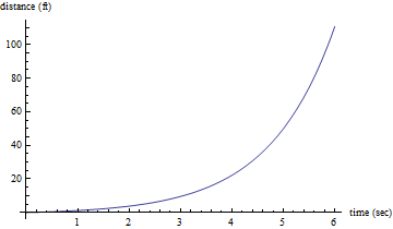
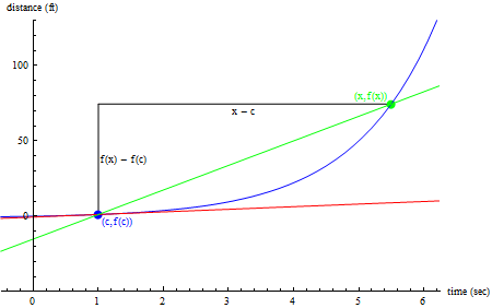
Let's consider a car that accelerates from zero to 60 mi/hr over a period of 6 seconds, traveling about 111 ft over that period of time. In this case, the car has gone an average of about 12.6 mi/hr (or 18.5 ft/sec, which we get from 111ft/6 sec). But this doesn't tell me much about how fast the car was going at any given moment because the car's speed is changing rapidly during that period of time. For example, at zero seconds the car was going 0 mi/hr, and for the first several seconds, it was not going much faster; but at six seconds, the car was going 60 mi/hr. But if all I can measure is the car's distance from the starting point at any given moment, how can I calculate the car's speed at any given moment, without resorting to an average speed?
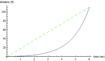
If we take a look at this graph, we can see that after 6 seconds, the car has gone about 111 ft total. This means that the average speed of the car over these 6 seconds is about 18.5 ft/sec (111 ft/ 6 sec), or about 12.6 mi/hr. In the next graph below, we can see the graph of our accelerating car again, this time with a green dashed line depicting the average speed of the car (i.e. a line which goes through the origin and has a slope of 18.5 ft/sec):
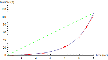
We can see that this line depicting the average speed over these six seconds is not a very good measure of how fast the car was actually traveling at any specific point in time: for example, at one second, the car was still going very slowly, and at six seconds, the car was actually traveling quite fast. For example, in the next graph below, we can see several things: the solid blue line still represents the car's distance over time; the dashed green line still represents the average speed of the car over these six seconds; and now there are also three red dotted lines whose slope represents the car's speed at 1.5 sec, 4 sec, and at 5.5 sec.
In this graph we can see that while the average speed of the car is pretty close to the car's speed at 4 seconds, the car's speed at 1.5 seconds is much slower than the average speed over the six-second interval, and the car's speed at 5.5 seconds is much faster than the car's average speed over that time period. To see for yourself how the instantaneous rate of change varies from the average rate of change throughout the whole six second interval, move the slider back and forth at the top of the figure below.
The slope of the red dotted line in the figure above shows the speed at each point on the curve as you move the slider back and forth. Notice how much this can vary from the average speed. Try to identify where this instantaneous speed is much faster or much slower than the average speed (i.e. where the red dotted line is much less steep or much more steep than the green dashed line), and where it seems to be the same.
It seems clear that in the example given in the above figures, calculating the average speed of the car isn't the most helpful technique if what we are really interested in is how fast the car is going at any given moment during that six seconds. What we really want is to be able to calculate theinstantaneous speed of the car at any given moment instead of the average overall speed.
So, in this case of a car that goes from 0 to 60 mi/hr in 6 seconds, the real question that we want to answer is, how did we know how to draw the red dotted lines? Their slopes are supposed to be the instantaneous speed of the car at each point as we drag the point along the curve, but we don't know how to calculate instantaneous speed because we can only calculate speed by finding the slope of the line between two points (i.e. the average speed between those two points).
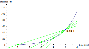
One natural idea is to try to approximate the instantaneous speed by calculating the average speed between the point we are interested in and another point that is really close. For example, if we want to know what the instantaneous speed is at five seconds, we could get closer and closer to the right answer by picking points closer and closer to x=5, and then calculating the average speed. This is illustrated in the next figure: here we can see that as we pick green points that are closer and closer to the blue point at x=5, and then draw a line through each point and the point at (5,f(5)), the slope of the line gets closer and closer to the instantaneous speed at x=5.
If we keep picking points that are ever-closer to the point on the curve where x=5, the slope of the line will get closer and closer to the instantaneous speed at the point where x=5.
To see for yourself how this works, consider the dynamic graph below of our car's motion. In this graph, the blue curve is our car's distance over time, the blue point labeled labeled (x0,f(x0)) is the point where we want to estimate the instantaneous speed, and the static (or unmoving) red line is what we might draw to describe the instantaneous speed of the car at the blue point just by "eyeballing" it.
Move the slider labeled x1 at the top of this figure back and forth: this will move the green point which has the label (x1,f(x1)) closer or farther away from the blue point (x0,f(x0)). The green line that constantly changes as you move the x1 slider is the line you get by connecting these two points, and you should be able to see that as you move the green point closer to the blue point, the slope of that green line gets closer to the instantaneous speed of the car at the blue point.
For example, when we let x0=5, which is the default in this figure, moving the green point closer and closer to the blue one shows us that the instantaneous speed of the car around 5 secs is pretty close to 40 ft/sec.
You can consider other values of x0 by moving the x0 slider bar on this figure. For example, if you move the x0 slider to where x0= 1 sec, you can see that the instantaneous speed at this time is pretty close to 1.72 ft/sec; and if you move the slider to where x0= 6 sec, you can see that the instantaneous speed at that time is pretty close to 88 ft/sec (which is equal to 60 mi/h, as we should expect from the original description of the car!).
So we can see that we can get closer and closer to the actual instantaneous speed at the blue point if the distance between the green and the blue points gets closer and closer to zero.
So what are the important things we should notice about this example?
When looking at a graph, the rate of change is depicted by the slope. So in order for us to understand how to calculate instantaneous rates of change, we need to have a good understanding of what slope is and how to interpret it.
Calculating an instantaneous rate of change exactly will require us to use limits, because calculating an instantaneous rate of change requires us to calculate what happens to the slope between two points on the graph as the distance between the two points approaches zero.
So, before we go further, let's begin by reviewing some of the basic properties of slope.
What we need to know about slope
Slope is a very important idea in calculus, so while it is a fairly simple concept, it makes sense for us to review some of the basic features of slope so that we can be sure that we understand this idea well. It is this idea of slope upon which many of these more complex calculus ideas will be based.
Slope (definition)
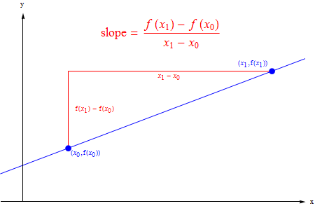
The slope of a line is a measure of the rate of change of y in terms of the rate of change of x. You have probably seen a number of different ways of looking at this in a previous class:
For two points (x0,y0) and (x1,y1), the slope can be calculated as:
(y0 - y1)/(x0 - x1),
or equivalently,
(y1 - y0)/(x1 - x0)
Graphically, this looks like this:
where the sign on the y-distance indicates whether one has to go up (positive) or down (negative) to go from (x0,y0) to (x1,y1), and the sign on the x-distance indicates whether one has to go to the right (positive) or to the left (negative) to go from (x0,y0) to (x1,y1).
We notice that a slope has two key pieces of information:
It's magnitude (i.e. how steep the line is - the bigger the magnitude of the slope, the steeper the line)
It's sign (i.e. whether the line is increasing or decreasing from left to right - lines with positive slopes have y-values that increase from left to right, and those with negative slope have y-values that decrease from left to right).
Basic Properties of Slope that will be Important for Calculus:
Before proceeding with the calculus concepts that follow, you should be comfortable with the following two major properties of slope:
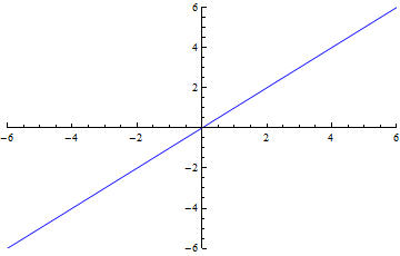
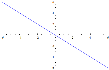
1) Sign of the slope (positive/negative)
If the line is increasing from left to right, it has a positive slope (because as we go up, in the positive y-direction, we also go to the right, in the positive x-direction, and dividing a positive by a positive gives us a positive). If the line is decreasing from left to right, it has a negative slope (because as we go down, in the negative y-direction, we also go to the right, in the positive x-direction, and dividing a negative by a positive gives us a negative).
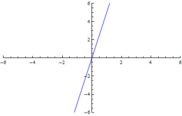
So this line has a positive slope:
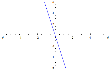
And this line has a negative slope:
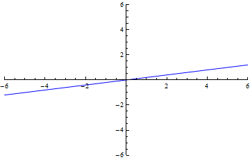
2) "Steepness", or the magnitude of the slope:
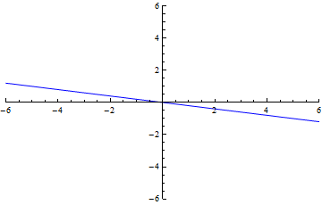
The steeper the line, the greater the magnitude of the slope. For example, in the table below, all the lines in the first row have positive slope, and all the lines in the second row have negative slope; but in both the first row and the second row, the slope of the lines get steeper as we move from left to right, because the magnitude of the slope in both cases gets larger.
But be careful with negative slopes!: While the lines in the second row get steeper as we go from left to right, the slopes actually get smaller because a negative number with a larger magnitude is actually smaller. For example, -1 has a smaller magnitude than -5 because -1 is closer to zero, but -5<-1 because -5 is to the left of -1 on the number line.
both lines have a slope that is not very steep
both lines have a slope that is steeper than the line to the left
both lines have a slope that is steeper than either line to the left
lines with positive slope
lines with negative slope
There are also a few other examples of what can happen with the "steepness" or magnitude of a slope:
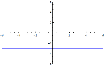
In the table below, the horizontal line to the left has a slope of zero. This makes sense because if we pick any two points on the line, the distance between the two y-values will always be zero (because all y-values on the graph are equal to -3), but the distance between the two x-values will always be something that is non-zero. Because zero divided by any non-zero number is zero, we can see that the slope must be zero.
In the table below, the vertical line to the right has a slope that is undefined. This makes sense because if we pick any two points on the line, the distance between the two x-values will always be zero (because all x-values on the graph are equal to 2.5). Because anything divided by zero will be undefined (remember we are not calculating a limit here, but an exact value, so indeterminate/determinate forms don't apply in this case), we can see that the slope must be undefined.
this line has a slope of zero
this line has a slope that is undefined
Calculating Instantaneous Rates of Change (Derivatives)
Now that we have both a firm understanding of both slopes and limits, we can now put these two ideas together to define the instantaneous rate of change of a function. We will call this instantaneous rate of change the derivative.
Derivative/instantaneous rate of change, Differentiability (definition)
The derivative, or instantaneous rate of change, of a function f(x) is the limit of the average rate of change between two points on the graph of f(x) as the distance between those two points approaches zero. We often use f '(x) to denote the derivative of f(x). Writing this out more formally, we get:
This equation means that if we want to find the instantaneous rate of change at x=c for f(x), we can calculate the slope between two points:(x,f(x)) and (c,f(c)), and then take the limit as x approaches c. The expression is just the slope of the line passing through these two points. We can see a visual representation of this relationship in the graph below. As the green point (x,f(x)) gets closer and closer to the blue point (c,f(c)), the slope will approach the slope of the red line (which represents the derivative of f(x) at x=c.
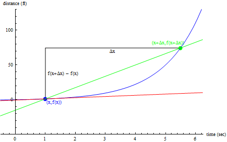
There is another way that we can write the same thing, but this time stressing a slightly different aspect of the relationship between the two points. If we label the point where we want to calculate the derivative (x,f(x)), we can then choose another point on the graph of f(x) just by picking some point that is a small distance away in the x-direction: We call that distance from (x,f(x)) in the x-direction Δx ("delta x"), and so the point on the graph which is Δx away from (x,f(x)) will be the point (x+Δx,f(x+Δx)). Be careful! Δx is one variable, even though it has two symbols that are used together to represent it: the symbol delta has no meaning on its own in this context, so be sure to treat Δx like one single variable.
This equation means that if we want to find the instantaneous rate of change at the point (x,f(x)), we can calculate the slope between two points:(x,f(x)) and anther point which is distance Δx away in the x-direction, (x+Δx,f(x+Δx)), and then take the limit as the distance between the two points Δx goes to zero. The expression is just the slope of the line passing through these two points. We can see a visual representation of this relationship in the graph below. As Δx shrinks, the green point (x+Δx,f(x+Δx)) gets closer and closer to the blue point (x,f(x)), and the slope will approach the slope of the red line (which represents the derivative of f(x) at x.
Be careful! We need to note that the variable x is playing a different role in the first definition of the derivative than in the second. In the firstdefinition of the derivative, the value c is staying fixed, and the variable x is varying. But in the second definition of the derivative, the value x is staying fixed, and the variable Δx is varying.
If the derivative f'(x) does NOT exist at a particular point x=c, then we say that the original function f(x) is NOT DIFFERENTIABLE at x=c.
If the derivative DOES exist for all x in some interval of values (a,b) (this just means for all x such that a<x<b), then we say that f(x) is DIFFERENTIABLE on the interval (a,b).
Secant line, Tangent line (definition)
The graphs above contain two different types of lines:
The green lines, which connected two points on the graph of f(x). A line like this that connects two points on a curve is called a secant line.
The red lines, which represented the instantaneous rate of change, instantaneous slope, or derivative of f(x) at a single point. A line that only passes through a single point of the curve (at least locally) and whose slope represents the derivative at that point is called at tangent line.
So we can see that we can use secant lines to approximate the tangent line at a point, and that if we take the limit of the slope of the secant line as the distance between the two points goes to zero, we can calculate the slope of the tangent line.
Examples:
Let's begin with an example where we try to find the derivative of a specific function at a specific point. Consider the following function, given in the graph of the animation below. Our function in this case is a parabola which opens upward, whose minimum is at x=2. For practice, let's try to think about what the derivative of this parabola is at several different points. The animation below shows us both the graph of the original function (in blue), and the slope of the line that passes through two points: the blue point (x0, f(x0)) which is a fixed point where we want to find the derivative, and the green point which is a distance of Δx away (in the x direction) from the blue point. We can gradually drag the Δx slider to decrease the distance between the green and blue points, and this will give us an estimate of the derivative at the blue point (x0, f(x0)). If we want to change the value of x0 (for example, changing it from x=1 to x=2), we can also adjust the slider labeled x0.
Use the animation below to try to estimate the derivative at:
x=1
x=2
x=3
To do this, first put the x0 slider at 1, and then drag the Δx slider until you can get the green and blue points as close together as possible without them actually being the same point (you will get an error message if you put them in the same spot because we can't calculate the slope of one point with itself - this will just give us 0/0 for the slope, which is undefined). Then, to do part b, move the x0 slider to 2 and repeat the process.
f(x) = 20x2 - 80x + 83
x0Δx
So, what did you get?
Using the animation, I estimated the following derivatives:
At x=1, f'(x) is about -39.6 (maybe it is actually -40?)
At x=2, f'(x) is about 0.08 (maybe it is actually 0?)
At x=3, f'(x) is about 39.76 (maybe it is actually 40?)
Now these are just estimates: I haven't actually calculated the derivative for this function using the equation for the function and the limit definition, so the actual derivative at each of these points is probably slightly different. For example, I might guess that the derivative at 1 is -40, at 2 is zero, and at 3 is 40 (although derivatives are not necessarily whole or even rational numbers, so this guess could be wrong). But it is good for me to use the graph to talk about what happens with the derivative because I can observe a number of important properties of the derivative that will help me to better understand what I am doing.
Below is an animation that shows us what the actually derivative is at each point: The slope of the red line at each point is the derivative at that point. Using this animation, find the exact value of the derivative at:
x=1
x=2
x=3
f(x) = 20x2 - 80x + 83
x0≅
We can see that in fact the derivative at these points is -40, 0, and 40 respectively. But we can also look at larger patterns for this derivative. We can see that as the value of x moves from 1 to 2 that the derivative is negative, and that it is getting less and less steep (or less and less negative). The derivative is then equal to 0 once x reaches 2, and as x moves from 2 to 3, the derivative is positive, and gets steeper and steeper as we move from left to right. So the derivative starts out as very negative number, gets progressively "less negative", hits zero, and then becomes positive and continually increases.
The Derivative as a Function
Instead of computing the derivative a different distinct points on a graph, we can think of the derivative itself as a function: It can be described by an equation which gives us the value of the derivative for f'(x) for each x-value that we plug into the equation.
Let's look at another animation that traces the value of the derivative for each value of x for the function f(x), and then graphs these values of the derivative on the y-axis for each x -value, this time on a new graph underneath. This animation gives us a picture of the original graph on the top in blue, and a picture of the values of the derivative of that original graph on the bottom in red.
f(x) = 20x2 - 80x + 83
x0≅
Slope of tangent line at x0: f'(x0) ≅
In this animation above, we can see that the derivative of this quadratic equation is a straight line which increases from left to right, and which crosses the x-axis at x=2. This makes sense, since the slope of f(x) was initially negative, got less and less negative as we moved from left to right, hit zero, and then became increasingly positive as we moved from left to right.
Let's look at the graph of a more complicated polynomial equation which has lots of local maximums and minimums, and let's think about what happens to the derivative as we go from left to right. Below is another animation that shows the original function at the top and the derivative at the bottom, this time for a fifth-order polynomial:
f(x) = 2x5 - x4 - 10x3 + x2 + 7x + 1
x0≅
Derivative at x0≅
When looking at this animation, here is what we see:
The derivative is positive, and getting less and less steep (or less and less positive, or smaller) as we move from the far left to about -1.5. Then, at about -1.5, where there is a local maximum, the derivative is zero. From about -1.5 to about -0.5, the derivative is negative, but we can see that from about -1.5 to about -1.2 the derivative is getting steeper (or more negative, or smaller), whereas from about -1.2 to -0.5, the derivative is getting less steep (or less negative, or larger). Then at about -0.5, where there is a local minimum, the derivative is zero. Similarly, from about -0.5 to 0.5, the derivative is positive, but from about -0.5 to 0 the derivative is getting steeper (or more and more positive, or larger), whereas from about 0 to 0.5 the derivative is getting less steep (or less and less positive, or smaller). Then, at about 0.5, where there is a local maximum, the derivative is zero. Now, from about 0.5 to 1.8, the derivative is negative again, but it is getting more steep from about 0.5 to 1.2 (or more and more negative, or smaller), and then getting less steep from about 1.2 to 1.8 (or less and less negative, or larger). The derivative is zero again at about 1.8 where we have a local minimum, and then the derivative is positive and getting steeper and steeper to the right of that.
Notice that we observed several important pieces of information about the derivative:
Where is the derivative positive, negative or zero?
Where is the derivative increasing (getting more positive or less negative) or decreasing (getting less positive or more negative)?
We have not yet seen it in two examples above, but there is also a third important question that we must also ask:
Where is the derivative undefined?
These three questions will be essential later when we use the derivative to solve a number of applied problems, and they will also be important in properly understanding the ideas behind the derivative. In the meantime, let's move on to looking at some examples where there is a point at which the derivative does not exist.
Does the derivative always exist?
Remember that the derivative is a limit, and since limits sometimes do not exist (for example, when they increase or decrease without bound, or when the limit is different on the left than on the right), there must be times when the derivative does not exist. In which cases can this happen? There are a couple of things that can go wrong:
The derivative is different when calculated from the left versus the right. Since the derivative is by definition a kind of limit, if the limit from the left and the limit from the right are different, the two-sided limit, and therefore the derivative, does not exist. Consider any graph that has a sharp (instead of gradual) turn, such as a cusp or a corner. Below is a graph with this kind of feature: it has a cusp at x=2. Use this animation to estimate the left-sided limit definition of the derivative and the right-sided limit definition of the derivative, by fixing the x0 value at 2, and by sliding the Δx slider back and forth, first moving the green point from the left towards 2, and then moving the green point from the right towards 2:
f(x) = |x3 - 8| + 3
x0≅Δx
Slope of secant line ≅
What did you get? Using the derivative limit definition from the left gave me a left-sided derivative of approximately -11.9, and using the derivative limit definition from the right gave me a derivative of about 12 in this case. We can see what the derivative might be more precisely at these points by looking at the animation below, which gives the derivative and its accompanying tangent line in red, for each point on the graph as we drag the slider back and forth which gives us the x value where the derivative is to be calculated.
f(x) = |x3 - 8| + 3
x0≅
Derivative of x0≅
Because the limit of the slope of the secant lines (as the green point approaches the red point), is different from the left and from the right at x=2, the derivative or two-sided limit does not exist in this case at x=2.
We can get a better idea of what the derivative function looks like by experimenting with the next animation. Try dragging the slider from the left to the right to see what the graph of the derivative will look like. Try to imagine in your mind first what you expect to see, before you drag the slider to the right:
f(x) = |x3 - 8| + 3
x0≅
Slope of tangent line at x0: f'(x0) ≅
By playing around with this animation, we can see that the derivative to the left of x=2 will be negative and getting steeper (or more negative, or smaller) from left to right, the derivative will be undefined exactly at x=2, and that the derivative will be positive and increasing from left to right to the right of 2.
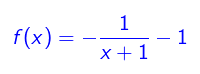
The tangent line is vertical. Since a vertical line has an undefined slope, if the slope in the derivative definition increases or decreases without bound as we take the limit, the derivative is undefined at that point.
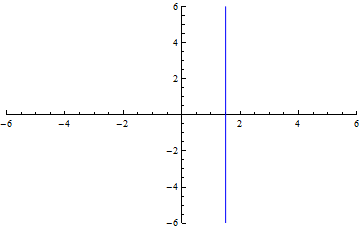
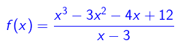
Consider the graph below. For this function, it looks like the slope will increase or decrease without bound as x approaches 3. Use the animation below to approximate the derivative at x=3:
x0≅Δx
Slope of secant line ≅
What did you find? We observe that as the green point moves closer and closer to the red point at x=3, the slope decreases without bound. Because the slope of f(x) approaches -∞ as x approaches 3, the derivative is undefined at x=3, a fact which we can see clearly in the next animation:
x0≅
Derivative of x0≅
The animation above again shows us more than just the derivative at x=3. It also shows us how the derivative behaves for all values of x. Once again let us try to first imagine what the graph of the derivative will look like, and then use the animation below to see if you were right:
x0≅
Slope of tangent line at x0: f'(x0) ≅
What patterns did you notice? We can see that the derivative here is negative everywhere on the graph, except at x=3 where it is undefined. But to the left of x=3, the slope of the original function is getting more and more negative (or decreasing) from left to right, whereas to the right of x=3, the slope of the original function is getting less and less negative (or increasing) from left to
Here is another example of a function which has a slope which will increase/decrease without bound at a particular point, in this case x=-1. In the example below, we can see that the slope of the function will increase without bound as we approach x=-1 from the left, and that it will decrease without bound as we approach x=-1 from the right. So the derivative at x=-1 will be undefined (because a vertical line has an undefined slope, and because when a limit approaches ±∞ it is undefined).
x0≅Δx
Slope of secant line ≅
x0≅
Derivative of x0≅
What would the actual graph of f'(x) look like? Think for a few moments and try to picture the graph of the derivative in your mind, and then use the following animation to graph the actual derivative to see if you were right:
x0≅
Slope of tangent line at x0: f'(x0) ≅
We can see from the animation above that the derivative of f(x) to the left of x=-1 will be positive, getting steeper or more and more positive (or increasing) from the left to the right, the derivative at x=-1 will be undefined, and that the derivative to the right of x=-1 will be positive but getting less steep or less and less positive (or decreasing).
We notice one key feature of this graph which we have not yet mentioned: f(x) is discontinuous at x=-1. While this is not the only reason that the derivative of f(x) is undefined at x=-1 in this example, it will turn out to be sufficient grounds for us to determine that the derivative is undefined, as we will see in the examples that follow. If the original function f(x) is discontinuous at a specific point, it will turn out that the derivative f'(x) does not exist at that point.
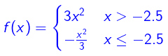
The original function f(x) is discontinuous at c. If the graph has some kind of break or jump at x=c, then the slope in the derivative definition will increase or decrease without bound as we take the limit at x=c.
Here we can see a classic example of a function that is discontinuous at a point: This function has a jump discontinuity at x = -2.5. Use the sliders to set x0= -2.5, and then move the Δx slider from the left towards x = -2.5, first from the left and then from the right. What value does the derivative approach from the left and from the right?
x0≅Δx
Slope of secant line ≅
What did you observe? As we approach from the left, the slope of the function approaches approximately 1.67. However, as we approach from the right, the slope of the function increases without bound as it becomes closer and closer to a vertical line. This happens because even though the x-values of the two points get closer and closer together, because of the jump discontinuity on the graph, the y-values will still remain some fixed distance apart (or more). So we can see that whenever we have a discontinuity at some point of f(x), we will always have this problem of the slope tending towards a vertical line, which will cause the derivative to be undefined at that point. Take a look at the following animation to see what the derivative will be of the graph at each point:
x0≅
Derivative of x0≅
Now once again try to imagine in your mind what the graph of f'(x) should look like in this case, and then use the animation below to check and see if you were right:
x0≅
Slope of tangent line at x0: f'(x0) ≅
We can see here that the derivative or slope of f(x) to the left of x = -2.5 will be positive and getting steeper or more positive (or increasing) as we go from left to right, the derivative will be undefined at x = -2.5, and the derivative to the right of x = -2.5 will be negative and getting less steep or less negative (or increasing) as we go from left to right.
Now let's consider one last kind of discontinuity: This graph has just a single point jump at x=1. Does the derivative exist at this point? Use the animation below to explore this idea, and try to decide what you think will happen to the derivative at x=1:
We can see that as the green point grows closer and closer to x=1 either on the right or the left, the slope between the two points approaches ±∞, and we get something that is closer and closer to t a vertical line. In much the same way as with the last function, we find that the derivative is undefined at x=1 for this case. We can now take a look at the following animation to see what the derivative will be of the graph at each point:
x0≅Δx
Slope of secant line ≅
And now we can use the animation below to think about what the graph of f'(x) will look like. As before, try to make an educated guess about the shape of the graph before you use the animation below to draw it for you:
x0≅
Slope of tangent line at x0: f'(x0) ≅
We can see that for this function, we can see that the derivative or slope is positive and increasing (getting steeper) everywhere except at x=1, where it is undefined. (Notice that in the animation above, the derivative has a small gap at x=1. Most graphing utilities won't show this, but this one has been rigged to show you precisely that there is a hole at x=1 in the derivative.)
In this lecture we have learned how to define the derivative as a limit, and how to use graphs to determine when the derivative does and does not exist, and to explore what the behavior of the limit will be more generally, not just at a single fixed point, but for any given value of x. Next we will work on finding equations for the derivative graphically, first by using the formal limit definition, and later by using patterns that we observe to come up with more general algebra rules for calculating the derivative.
However, as we move on to calculate limits algebraically, it is very important to keep this graphical picture of what the derivative really is in mind. The rest of this course will focus on a number of different applications of derivatives, and in order for us to solve those problems correctly, we will need a good intuitive and graphical understanding of what the derivative is, in addition to algebra techniques for calculating equations for the derivative.