What is Calculus?
By the end of this lecture, you should be able to briefly explain the underlying questions which motivated the development of calculus, and to very briefly explain how the informal defintion of a limit relates to these questions.
To understand what calculus is, it may help us to begin by looking at two questions that motivated the creation of calculus. These two questions cannot be answered using only algebra and geometry; we need a new mathematical theory to answer them. And this new theory that we will develop in order to answer these questions is what we call calculus.
-
How can we calculate an instantaneous speed (or rate of change) rather than just an average speed?
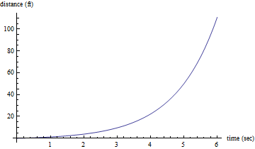
For example, let's consider a car that accelerates from zero to 60 mi/hr over a period of 6 seconds, traveling about 111 ft over that period of time. In this case, the car has gone an average of about 12.6 mi/hr (or 18.5 ft/sec, which we get from 111ft/6 sec). But this doesn't tell me much about how fast the car was going at any given moment. For example, at zero seconds the care was going 0 mi/hr, and for the first several seconds, it was not going much faster; but at six seconds, the car was going 60 mi/hr. But if all I can measure is the car's distance from the starting point at any given moment, how can I calculate the car's speed at any given moment, without resorting to an average speed?

-
How can we calculate the area under a curve rather than just the area of more "regular" objects like squares, triangles, circles, and regular polygons?
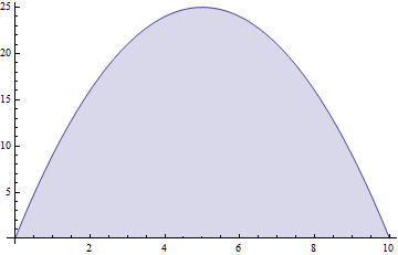
For example, if I want to determine the exact area of the following shape, I can't use any of the techniques that I've already learned in algebra or geometry to do this, because this shape is not a circle, triangle, regtangle or a regular polygon, and it can't be broken down into a finite set of these regular shapes. But there are plenty of cases in real life where I might need to know the area of more irregular shapes (for example, if I need to manufacture a bunch of these as part of some machinery, I need to know how much material I will need to make each one). So how can I calculate the exact area of this shape?

In order to answer these two questions, we need similar tools. Let's look at these two questions in more detail to get an idea of how we might approach these kinds of problems:
1) How can we calculate an instantaneous speed (or rate of change) rather than just an average speed?
To consider this question, let's start with a simple example. In this graph, a car accelerates quickly from 0 to 60 mph:

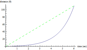
If we take a look at this graph, we can see that after 6 seconds, the car has gone about 111 ft total. This means that the average speed of the car over these 6 seconds is about 18.5 ft/sec (111 ft/ 6 sec), or about 12.6 mi/hr. In the next graph below, we can see the graph of our accelerating car again, this time with a green dashed line depicting the average speed of the car (i.e. a line which goes through the origin and has a slope of 18.5 ft/sec):

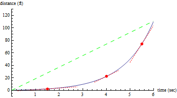
We can see that this line depicting the average speed over these six seconds is not a very good measure of how fast the car was actually traveling at any specific point in time: for example, at one second, the car was still going very slowly, and at six seconds, the car was actually traveling quite fast. For example, in the next graph below, we can see several things: the solid blue line still represents the car's distance over time; the dashed green line still represents the average speed of the car over these six seconds; and now there are also three red dotted lines whose slope represents the car's speed at 1.5 sec, 4 sec, and at 5.5 sec.

In this graph we can see that while the average speed of the car is pretty close to the car's speed at 4 seconds, the car's speed at 1.5 seconds is much slower than the average speed over the six-second interval, and the car's speed at 5.5 seconds is much faster than the car's average speed over that time period. To see for yourself how the instantaneous rate of change varies from the average rate of change throughout the whole six second interval, move the slider back and forth at the top of the figure below.
The slope of the red dotted line in the figure above shows the speed at each point on the curve as you move the slider back and forth. Notice how much this can vary from the average speed. Try to identify where this instantaneous speed is much faster or much slower than the average speed (i.e. where the red dotted line is much less steep or much more steep than the green dashed line), and where it seems to be the same.
It seems clear that in the example given in the above figures, calculating the average speed of the car isn't the most helpful techique if what we are really interested in is how fast the car is going at any given moment during that six seconds. What we really want is to be able to calculate the instantaneous speed of the car at any given moment instead of the average overall speed.
Instantaneous Rate of Change (informal definition)
An instantaneous rate of change is the rate of change at a single point on a graph.
(Speed is really just one example of a rate of change: specifically the rate at which distance changes over time. So we can also talk about an instantaneous speed, for example.)
Since a rate of change by definition requires us to take the change in y over the change in x, at first this definition doesn't seem to make sense from a mathematical perspective - how can we have a rate of change at a single point? Don't we by definition need two points to calculate a rate (i.e. change in y divided by change in x)? To address this problem, we are going to have to invent a new mathematical theory, and it is this new theory that we will call calculus. Once we've done that, we will come back and write out a formal definition. But for now, we all have an intuitive sense of what it might mean to have a rage of change a single point: For example, if I am driving in a car I understand intuitively what it means to say that I am going at 25 mi/hr at this exact instant as I am in the process of accelerating from 0 to 60 mi/hr (even if I am not sure how to calculate it). So for now, just to have someplace to start, we are going to rely on this intuitive picture in our minds to talk about this term instantaneous speed, while at the same time recognizing that in order to really do any proper mathematics with this term, we will have to formally define it first.
So, in this case of a car that goes from 0 to 60 mi/hr in 6 seconds, the real question that we want to answer is, how did we know how to draw the red dotted lines? Their slopes are supposed to be the instantaneous speed of the car at each point as we drag the point along the curve, but we don't know how to calculate instantaneous speed because we can only calculate speed by finding the slope of the line between two points (i.e. the average speed between those two points).
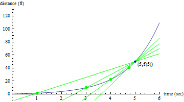
One natural idea is to try to approximate the instantaneous speed by calculating the average speed between the point we are interested in and another point that is really close. For example, if we want to know what the instantaneous speed is at five seconds, we could get closer and closer to the right answer by picking points closer and closer to x=5, and then calculating the average speed. This is illustrated in the next figure: here we can see that as we pick green points that are closer and closer to the blue point at x=5, and then draw a line through each point and the point at (5,f(5)), the slope of the line gets closer and closer to the instantaneous speed at x=5.

If we keep picking points that are ever-closer to the point on the curve where x=5, the slope of the line will get closer and closer to the instantaneous speed at the point where x=5.
To see for yourself how this works, consider the dynamic graph below of our car's motion. In this graph, the blue curve is our car's distance over time, the blue point labeled labeled (x0,f(x0)) is the point where we want to estimate the instantaneous speed, and the static (or unmoving) red line is what we might draw to describe the instantaneous speed of the car at the blue point just by "eyeballing" it.
Move the slider labeled x1 at the top of this figure back and forth: this will move the green point which has the label (x1,f(x1)) closer or farther away from the blue point (x0,f(x0)). The green line that constantly changes as you move the x1 slider is the line you get by connecting these two points, and you should be able to see that as you move the green point closer to the blue point, the slope of that green line gets closer to the instantaneous speed of the car at the blue point.
For example, when we let x0=5, which is the default in this figure, moving the green point closer and closer to the blue one shows us that the instantaneous speed of the car around 5 secs is pretty close to 40 ft/sec.
You can consider other values of x0 by moving the x0 slider bar on this figure. For example, if you move the x0 slider to where x0= 1 sec, you can see that the instantaneous speed at this time is pretty close to 1.72 ft/sec; and if you move the slider to where x0= 6 sec, you can see that the instantaneous speed at that time is pretty close to 88 ft/sec (which is equal to 60 mi/h, as we should expect from the original description of the car!).
So we can see that we can get closer and closer to the actual instantaneous speed at the blue point if the distance between the green and the blue points gets closer and closer to zero.
2) How can we calculate the area under a curve rather than just the area of more "regular" objects like squares, triangles, circles, and regular polygons?
To consider this example, let's go back to our original graph of a simple shape that is bounded by a parabola on the top and the x-axis on the bottom:

If we want to find the area of the shaded region above, where should we start?
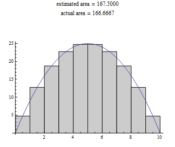
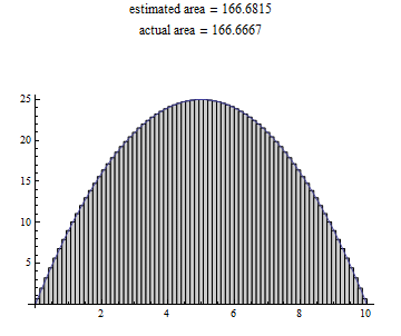
One option which is similar to what we did in our attempt to answer question 1 is to begin by trying to approximate the shaded area under the parabola. So, for example: we know how to find the area of rectangles quite easily, so we could fill the area under the curve with a bunch of little rectangles, and then add up the area of all the rectangles, something like this:

Here we have decided to make the height of each rectangle the same as the height of our curve at the midpoint of the rectange, and we have made all our rectangles the same width, to keep things simple. We can see that the estimated area here is pretty close to the actual area (you'll just have to trust us on the actual area right now, since we don't yet know how to calculate it :)).
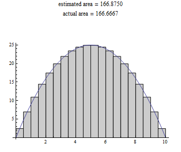
But is there a way that we could get a better estimate? What if we made the rectanges much narrower, and used more of them, like this?

This makes our estimate even better! What if we shrink the width of the rectangles even more?

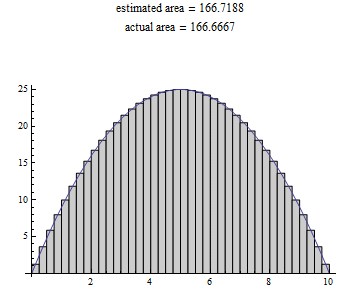
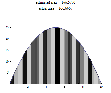
Getting closer and closer... Now shrinking those rectangle widths even more:

Even more improvement, so let's try shrinking those rectangle widths even more, one last time:

To see this more clearly for yourself, you can experiment with the interactive graph below. In the figure below, move the slider left and right: this will decrease or increase the number of rectanges (thereby increasing or decreasing the width of those rectangles). While you manipulate the number of rectangles used to estimate the area under the curve, watch how this affects how close the estimated area comes to the exact area under the curve. (If you want to play around with other curves, you can also hit some of the other function buttons and experiment with these alternate functions in the same way.)
We can see from these images that we can get closer and closer to the actual area under the curve if the width of the rectangles gets closer and closer to zero.
So where do these new calculus theories come in?
What we've done so far is really just to use algebra to try to approximate certain things (such as instantaneous speed at a point on a graph or area under a curve) that we'd actually like to know exactly. The whole reason calculus was invented was because we are willing to invent a new area of math if it will let us do these calculations exactly instead of just using algebra to approximate what we want.
If we look closely, we can see that the two questions which we explored above have one thing in common:
As a certain input value gets closer and closer to zero, our approximation of a particular outcome value gets closer and closer to the exact value.
This pattern leads us to a definition that will be the foundation of calculus:
Limit (informal definition)
If f(x) eventually gets closer and closer to a specific value L as x approaches a chosen value c from the right, then we say that the limit of f(x) as x approaches c from the right is L.
If f(x) eventually gets closer and closer to a specific value L as x approaches a chosen value c from the left, then we say that the limit of f(x) as x approaches c from the left is L.
If the limit of f(x) as x approaches c is the same from both the right and the left, then we say that the limit of f(x) as x approaches c is L.
It is important to notice that this is an "informal" definition: this means that there are some words in this definition that aren't precisely defined enough in order for this to be a formal math definition, because they could be interpreted to mean several different contradictory things, depending on how we interpret them. For now though, just to get started thinking about what limits might look like, we will use this definition. Once we have developed some intuition about what a limit really is, we will come back and formulate a proper formal definition.
So calculus is the area of mathematics where we solve problems using limit processes. This means that calculus is based on using the definition of a limit to calculate exact values for things such as instantaneous speed or the area under a curve, rather than simply using algebra to approximate these values.
Limit processes and calculus can actually be used to answer a whole range of questions beyond the two questions initially posed here; the two questions used in this lecture have been chosen specifically becuase they are the foundation for most of the calculus techniques used in a first year college calculus course (the first question is the main motivating question for the first semester, and the second question is the main motivating question for the second semester). However, here is a sample of some other questions that can be answered using calculus and limit processes:
-
How do we find the maximum or minimum height of a curve in any given area of a graph?
-
How do we measure the curvature of a curve at a particular point?
-
How do we find the direction of motion along a curve?
-
How do we find the length of an arc, or curve segment?
-
How do we find the volume or surface area of certain types of objects whose boundaries are defined by curves rather than more regular shapes like lines, rectanges, or circles?
-
How do we find the "center" of a two-dimensional region that isn't a rectangle or other "regular" shape?
-
How do we find the work done by a force that varies over time or by location; or the mass of a solid whose density is not uniform throughout (i.e. more dense in some regions than others)?
In the next lecture, we will explore this informal definition of limits so that we can better understand it and so that we can learn how to use it to solve problems.
